Here are some new features included in the latest update, deployed on 6/20/2020.
Color of the graph reflects the time scale of the displayed window
When you are zoomed in viewing shorter time spans, you’ll see the graph rendered as an orange/beige color. As you zoom out, the graph becomes more blue. (Inspired by the physical phenomenon of mountains appearing to be more blue when they are farther away)
Note that the color gradient change is logarithmic, since we are dealing with timespans ranging from a few days to billions of years! So, you won’t see dramatic change using the incremental zoom in/out tool. The effect is most interesting when jumping forward and backward to higher and lower resonances.
Fractal dimension calculation
I thought it might be interesting to figure out the fractal dimension of the timewave. I implemented an algorithm that treats the graph as a coastline and measures with subsequently smaller rulers (this video shows how the process works).
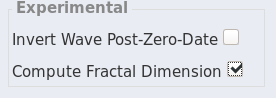
If you enable the option in the left-hand pane, the fractal dimension will be computed for the window you’re currently viewing. You’ll see the result of the computation in the lower pane:
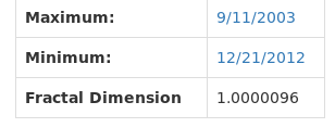
I don’t have any external validation of the code, nor do I believe the computation has been done anywhere before, so I can’t be 100% sure of its accuracy. However, as you move around the graph, it stays very close to 1, which seems intuitively correct.
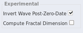
Option to invert the graph post-zero-date
 Since nothing much interesting happens when you scroll to the right of the zero date, and considering the fact that we are currently existing in the time after Terence McKenna’s original zero date designation, perhaps we should consider ideas for extending the wave past it.
When enabled, this feature takes the wave and rotates it 180 degrees on the plane around the zero point. The effect is that at the zero date, the graph descends below the x-axis, and extends indefinitely into the future.
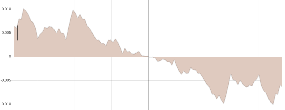
This operation actually mimics a step early in the process of constructing the number set from which the wave is generated. Namely, the 180 degree rotation of the graph of the First Order Differences in which the the graph is rotated and overlayed atop itself. Of course, the major difference is that in this operation we aren’t overlaying the rotated graph on top of itself; rather we are appending it to the end. However, I believe it does create a beautiful symmetry in the overall process, as we’re kind of unraveling that earlier step. (probably this warrants a little more explanation/exploration!)
Other back-end changes
Finally, it is not visible on the user interface, but worth noting anyway: I included some changes in this update that refactored the hard-coded number sets (Kelley, Watkins, Sheilak, and Huang Ti) separating them out into their own database objects, creating a more “pluggable” framework for using different number sets. This will enable a future feature wherein the user can experiment with uploading and graphing with different numbersets beyond the original four. This will enable the user to experiment with tweaking the process by which McKenna et. al. actually derived the set and observing the effect on the graph.