Categories
Uncategorized

Setting up a Dev environment

The Timewave Explorer application is fully free and open source, and is built on a platform of my own creation called Noonian, also fully free and open source.

Unfortunately the documentation is pretty sparse, particularly for building and installing packages, and for setting up and collaborating on a project with source control (git).  So if you want to mess around with the dev side of this Timewave Explorer, it’ll take a little hacking.

For this post, I’ll make available a simplified method for setting up a dev envionment for anyone who’d like to poke around and modify the source code.

Note, the following was done on a Debian Linux commandline.  It should work pretty much the same on a Mac OS machine (there may be some wrinkles to deal with), but on a Windows machine there’s probably more wrinkles than its worth wrestling with.  If you’re using windows and aren’t in the mood for those struggles, I’d suggest setting up a Debian virtual machine on VirtualBox and using that.  (I’d also recommend switching to Linux entirely and getting the hell away from the Microsoft and Apple tech overlords!  But that’s a discussion for another time.)

Here are the steps:

  1. Set up the Noonian stack (namely MongoDB, Node.js, and Noonian itself) according to these instructions.
    1. Stop at “Instance Setup” step, as I’m providing the instance directory in a zip file below.
    2. Before proceeding, make sure the mongo service is running, and node and noonian are available on the PATH:
      1. echo show databases | mongo
        node -v
        noonian -h
  2. Grab this zip file which contains the fully configured instance, as well as a dump of the bootstrapped DB.  Unzip to a directory on your hard drive, and change directory to make it your current working directory (all commands below should be executed from within this directory)
  3. Restore the database dump to mongo DB
    1. mongorestore --db noonian-twz-dev mongodump/2021-03-03/
  4. Tell noonian about the instance and start it up
    1. noonian add
      noonian start
  5. Load it up in your browser; Log in to the back-end with username admin (password is admin)
    1. The timewave explorer application:
      1. http://127.0.0.1:6500/twz-dev/twz_browser.html
    2. The development back-end:
      1. http://127.0.0.1:6500/twz-dev/dbui2/index/

To start your journey into the code, Go to Angular -> Applications and load up “twz_browser.html“.

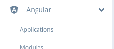
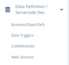
The Angular templates, controllers, directives and such that make up the web application are accessible via that same Angular submenu. Server-side components are accessible via the Data Definition / Serverside submenu, primarily the “Web Services” and “CodeModules”.

Hopefully that gets you started!  Feel free to comment on this post with questions/problems.


Categories
Uncategorized

Update v0.5.0

Here are some new features included in the latest update, deployed on 6/20/2020.

Color of the graph reflects the time scale of the displayed window

When you are zoomed in viewing shorter time spans, you’ll see the graph rendered as an orange/beige color.  As you zoom out, the graph becomes more blue.  (Inspired by the physical phenomenon of mountains appearing to be more blue when they are farther away)

Note that the color gradient change is logarithmic, since we are dealing with timespans ranging from a few days to billions of years!  So, you won’t see dramatic change using the incremental zoom in/out tool.  The effect is most interesting when jumping forward and backward to higher and lower resonances.

Fractal dimension calculation
“Experimental” features can be enabled in left-hand pane

I thought it might be interesting to figure out the fractal dimension of the timewave.  I implemented an algorithm that treats the graph as a coastline and measures with subsequently smaller rulers (this video shows how the process works).

If you enable the option in the left-hand pane, the fractal dimension will be computed for the window you’re currently viewing.  You’ll see the result of the computation in the lower pane:

Right-hand side of the pane below the graph

I don’t have any external validation of the code, nor do I believe the computation has been done anywhere before, so I can’t be 100% sure of its accuracy.  However, as you move around the graph, it stays very close to 1, which seems intuitively correct.

Option to invert the graph post-zero-date

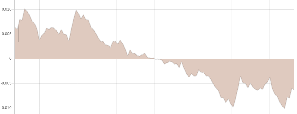
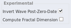
Since nothing much interesting happens when you scroll to the right of the zero date, and considering the fact that we are currently existing in the time after Terence McKenna’s original zero date designation, perhaps we should consider ideas for extending the wave past it.

When enabled, this feature takes the wave and rotates it 180 degrees on the plane around the zero point.  The effect is that at the zero date, the graph descends below the x-axis, and extends indefinitely into the future.

the graph extending 10 years before and after the zero date, with the feature enabled

This operation actually mimics a step early in the process of constructing the number set from which the wave is generated.  Namely, the 180 degree rotation of the graph of the First Order Differences in which the  the graph is rotated and overlayed atop itself.  Of course, the major difference is that in this operation we aren’t overlaying the rotated graph on top of itself; rather we are appending it to the end.  However, I believe it does create a beautiful symmetry in the overall process, as we’re kind of unraveling that earlier step.  (probably this warrants a little more explanation/exploration!)

Other back-end changes

Finally, it is not visible on the user interface, but worth noting anyway: I included some changes in this update that refactored the hard-coded number sets (Kelley, Watkins, Sheilak, and Huang Ti) separating them out into their own database objects, creating a more “pluggable” framework for using different number sets.  This will enable a future feature wherein the user can experiment with uploading and graphing with different numbersets beyond the original four.    This will enable the user to experiment with tweaking the process by which McKenna et. al. actually derived the set and observing the effect on the graph.

Categories
blog

Background

I read The Invisible Landscape (1993 edition) a couple years ago, hoping to get insight into this mysterious and elusive Timewave Zero concept I had heard about while exploring McKenna material online.  It wasn’t exactly light reading (much of the biological and DNA discussion zoomed miles over my head), and it took awhile to get to the content I was looking for, but those last few chapters were illuminating.

I felt I got the gist of the mechanics of the Timewave’s derivation from the I Ching, and spent a little time messing around with the first steps (plotting the “First-Order Differences” to draw the “Simple Wave”).  However, I hit a little snag at one point of the derivation, after which I decided to switch focus to start building software to actually graph the Timewave.  I was grateful to have found John Phelps’ public domain implementation of the fractal transform algorithm, which I translated into Javascript and proceeded to build a web-based graphical user interface around.

Like with many of my projects, I reached a certain point and ran out of steam, set it aside and let it gather dust on my hard drive.  Earlier this year, I decided it’s time to pick it back up after seeing a video by Alan Abadessa-Green, the end of which he mentions Timewave Zero.

So here we are!  I got the software to a state of functionality I was willing to share, deployed it and created this site and a video to go with it, and posted a message to reddit to invite folks to come check it out.  My plan after that was to follow up by creating some documentation, but wouldn’t you know it, I got sucked back into the theoretical stuff.

You see, the technical description at the end of the Invisible Landscape left me believing I had grasped the basics of the derivation of the 384-integer numberset that serves as the basis for the timewave graph.  (I never needed to know the details of that derivation in order to build the Timewave Explorer software; for that I could just plop in the already-derived numbers.)  I figured that eventually I’d sit down with a pen an paper, study the relevant chapters a little more carefully, and would be able figure it out in an hour or two.

Yowzer was I wrong about that.  It turns out that the Invisible Landscape doesn’t provide enough information to derive the numberset!  I went digging online and found technical information to be very sparse.  However, I was determined to crack the nut, and I am happy to say I’ve powered through it and have successfully derived the Kelley and Watkins numbersets, and now have a solid understanding.

My plan moving forward is this: to document these technical details in a comprehensive and intelligible fashion by creating a series of videos and articles.  I will walk the viewer step-by-step starting with the I Ching all the way to the timewave, with careful attention to the intuition of each step – articulating both the how and the why.  All spreadsheets, data, documents, sourcecode, etc. will be available alongside the explanations, so anyone will be able to go in and review every detail.  That way the next person who comes along with my level of curiosity doesn’t have to spend quite so much time and energy pulling it all together!


Stay tuned!

Gene